Bisection
Method - Half-interval Search
This
code calculates roots of continuous functions within a given interval
and uses
the Bisection method. The program assumes that the provided points
produce a
change of sign on the function under study. If a change of sign is
found, then
the root is calculated using the Bisection algorithm (also known as the
Half-interval Search). If there is no change of sign, an error is
displayed.
You could try with other low or high values, or you could improve the
code to
find two values with a different sign before going on.
In
general, when we work with numerical methods we must be aware that
errors may
result for a number of reasons. First, a root may be calculated when it
should
not be. It could happen if a point is so close to zero that a root is
found due
to round-off error. Second, two roots may be so close together that the
program
never finds the opposite signs between them...
You
will provide the function, the interval (both low and high values) and
a
tolerance. This suggested version of the method will list the evaluated
intervals and the final approximation found using your tolerance.
function
m = bisection(f, low, high, tol)
disp('Bisection
Method');
%
Evaluate both ends of the interval
y1 =
feval(f, low);
y2 =
feval(f, high);
i = 0;
%
Display error and finish if signs are not different
if y1 * y2
> 0
disp('Have not found a change
in sign.
Will not continue...');
m
= 'Error'
return
end
%
Work with the limits modifying them until you find
%
a function close enough to zero.
disp('Iter
low
high
x0');
while
(abs(high - low) >= tol)
i
= i + 1;
% Find a new value to be
tested as a root
m = (high + low)/2;
y3
= feval(f, m);
if y3 == 0
fprintf('Root at x = %f \n\n', m);
return
end
fprintf('%2i \t %f \t %f \t %f \n', i-1,
low, high, m);
% Update the limits
if y1 * y3 > 0
low = m;
y1 = y3;
else
high = m;
end
end
%
Show the last approximation considering the tolerance
w
=
feval(f, m);
fprintf('\n
x
= %f produces f(x) = %f \n %i iterations\n', m, y3, i-1);
fprintf('
Approximation with tolerance = %f \n', tol);
Let’s
say that we want to find a root of the function
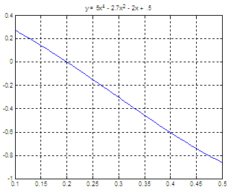
y = 5x4 - 2.7x2 - 2x + 0.5
and want to explore the
interval [0.1, 0.5], we could call
the function from another m-file, like this:
my_fun =
@(x) 5*x^4 - 2.7*x^2 - 2*x + .5;
low =
.1;
high =
0.5;
tolerance
= .00001;
x =
bisection(my_fun, low, high, tolerance);
the result is:
Bisection Method
Iter
low
high
x0
0
0.100000 0.500000
0.300000
Root at
x = 0.200000
If we plot the function,
we get a visual way of finding
roots. In this case, this is the function

Now,
another example and
let’s say that we want to find the
root of another function
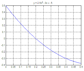
y = 2.5x2
- 3x + 0.5
using another interval,
like [0, 0.5], we can use this code
to call the half-interval search
my_fun =
@(x) 2.5*x^2 - 3*x + .5;
low = 0;
high =
0.5;
tolerance
= .00001;
x =
bisection(my_fun, low, high, tolerance);
and we get this
information from the proposed code above:
Bisection Method
Iter low
high
x0
0 0.000000
0.500000
0.250000
1 0.000000
0.250000
0.125000
2 0.125000
0.250000
0.187500
3 0.187500
0.250000
0.218750
4 0.187500
0.218750
0.203125
5 0.187500
0.203125
0.195313
6 0.195313
0.203125
0.199219
7 0.199219
0.203125
0.201172
8 0.199219
0.201172
0.200195
9 0.199219
0.200195
0.199707
10 0.199707
0.200195
0.199951
11 0.199951
0.200195
0.200073
12 0.199951
0.200073
0.200012
13 0.199951
0.200012
0.199982
14 0.199982
0.200012
0.199997
15 0.199997
0.200012
0.200005
x = 0.200005
produces
f(x) = -0.000009
15
iterations
Approximation
with
tolerance = 0.000010
Again,
plotting the function is a good idea to better know what we’re doing...

Maybe you're also interested in:
Finding
intersections
Other
ideas
about root finding
Nonlinear
systems
From
'Bisection Method' to home
From
'Bisection Method' to Generic Programming with Matlab

|


