Curve Fitting for experimental data

In this experiment, we are going to explore another built-in function in Scilab intended for curve fitting or finding parameters or coefficients. Its name is ‘datafit’. Naturally, you can see all the possibilities and uses of the function if you type “help datafit” on your command window. The online reference manual should always be your first source of information.  

We are going to use the simplest case for fitting a curve to given or found data. 

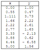
Let’s say that we have collected some results from an experiment. These are the specific numbers 

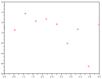
If we graph the table in Scilab, we’re going to get this plot  

Now, let’s say that we know in advance that those measured or somehow collected points in our experiment are part of a nonlinear function of this type: 

Our mission is to find the parameters C₁, C₂ and C₃. 
 

We know that the function datafit is used for fitting data to a model. For a given function G(p, z), this function finds the best vector of parameters p for approximating G(p, z_i) = 0 for a set of measurement vectors z_i. Vector p is found by minimizing G(p, z₁)' WG(p, z₁) + G(p, z₂)' WG(p, z₂) + ... + G(p, z_n)' WG(p, z_n)  

where 

• G is a function descriptor
• W is a weighting matrix

datafit is an improved version of fit_dat, also available in Scilab.

The first step in our demonstration is to create a file (called OF_datafit1.sci) that includes our parameterized function (in this case called data_fit_1) and our way to measure the error (in this case the function is called myerror). 
 

This is one way to do it:  

// This function takes vector x and the parameters 
// of the function
function y = data_fit_1(x, c)
  y = exp(c(1)*x) .* cos(c(2)*x) + c(3)*sin(x);
endfunction 

// This is a way to measure the error, to find the least one.
// The error function will call the parameterized function.
function e = myerror(c, z)
  x = z(1); y = z(2);
  e = y - data_fit_1(x, c);
endfunction 

Now, we can create a main script that can use the function datafit and the input data. One way to do it is like this:  

// Clear windows, memory and screen
xdel(winsid()); clear; clc 

// Load our functions into memory
getf('OF_datafit1.sci'); 

// Measured data in vectors x and y
x = [0 0.55 1.11 1.66 2.22 ...
     2.77 3.33 3.88 4.44 5];
y = [1 0.47 3.73 2.22 2.61 ...
     1.63 -2.13 0.62 -6.58 1.56]; 

// Plot the original data
plot(x, y, 'ro') 

// Prepare vector z with given coordinates
z = [x; y];
// This is our first attempt to find the parameters
c0 = [2 2 2]'; 

// copt is supposed to be the best result
// err is the value of the error at the end of the process
[copt, err] = datafit(myerror, z, c0); 

// Let's see how good our optimization resulted
x = linspace(0, 5, 100);
y = data_fit_1(x, copt);
plot(x, y)

This is the result:  

err = 43.654725
copt =
    0.1361701
    2.3429071
    2.5378073

It was a nice try, but the error was very high (it should be close to zero) and our result was not good at all.

We could manually try different values in c0, the starting point. We can expect Scilab to deliver different results if we enter different seeds as starting points...
 

Let’s try a different approach. We’re going to create a loop of 10 iterations. We can create a random vector for c0 (the seed) each time, and we are going to take the best result after those 10 attempts. It’s another way of approaching the problem, instead of going one vector at a time...
 

I can suggest something similar to this code...
 

// Let’s try random starting seeds between -5 and 5
a = -5; b = 5;
for k = 1 : 10
  c0 = a + (b - a)*rand(3, 1);
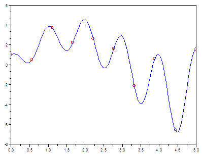
  [copt(:, k), err(k)] = datafit(myerror, z, c0);
end 

// The least error after 10 trials is
[m, k] = min(err)
copt = copt(:,k) 

// Let’s plot the best found result
x = linspace(0, 5, 100);
y = data_fit_1(x, copt);
plot(x, y)

And we get this result... 

k  = 3
m  = 0.0030935
copt  =
    0.3006878
    6.3193538
    3.0024572
 

Much better..., now our function has an error of only 0.003 (found in the third iteration) and the best found coefficients produce a function that hits the experimental data almost perfectly. 

Mission accomplished!
 

Maybe you're interested in

Polynomial Fit

Least Squares Fit