
Exponential Regression - calculate with MatlabWe’ll work this time with exponential regression in a curve fitting example. The following codes find the coefficients of an equation for an exponential curve.
You must provide the x
and y coordinates for known data
points. Once the curve has been fitted
you may predict values of y = f(x)
for given values of x. We’re going to experiment with three different methods to cope with our exponential regression.
Example: The
table below shows the number of strange particles present in a
scientific
experiment at various points in time. We have to fit an exponential
curve to
the data and estimate the number of particles after 7 hours. number
of hours = [0 1 2 3 4 5 6] First
method: using known formulas
We know
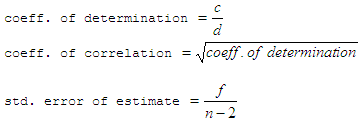
that coefficients a and b are determined by  where n = number of points in given
data
We also
know that  where  Then,
this is easy to code... clear,
clc, close all, format compact, format
long %
enter data %
calculate coefficients a and b %
calculate coeff. of determination, coeff. of correlation %
We can calculate any point along the curve The
results are: b
= 0.42237507956752 Interpolation:
7 Second
method: optimization techniques with fminsearch
This is
a very powerful technique that can be applied in curve fitting,
exponential
regressions, or nonlinear problems in general. We can obtain the
coefficients
without
knowing the formulas above! What we
do is set the problem in such a way that it can be minimized. The term
‘minimization’ means that we’re comparing our guesses against the given
data. The
least error, after several automatic iterations, is going to be the
solution to
our problem. Matlab built-in function fminsearch tries different
coefficients
and stops when the least error has been found. Let’s
say that we prepare this objective-function: function U =
OF_exp_regr(c) %
try coefficients %
try to match original data, and return difference We can
now use that objective with the following code: clear,
clc, close all, format compact %
enter data and plot it %
enter starting point: before optimization %
launch optimization method %
plot results after optimization The results are:
c
= 24.88778378033923 0.42303260089823
You
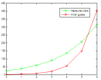
see? We started with a
= 1 and b
= 1 (as in c0 = [1 1]), and we got the initial
graphic. The green line is the target, the red line is our initial
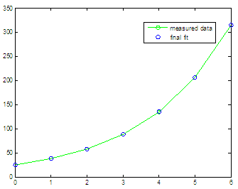
guess. After
the optimization process we got c(1)= a = 24.8877
and c(2)=
b
= 0.4230, and those
coefficients produced the second plot, with green target and blue
points showing our
fit. The results are quite similar to those found by the method using
formulas,
right? Third
method: inter/extrapolation
This
method doesn’t provide results for coefficients, but it an example of
interpolation and extrapolation capabilities in Matlab. We’ll
use buil-in function interp1, whose basic syntax is: yi = interp11(X,
Y, XI, METHOD, 'extrap') uses the specified method for Methods,
among others, can be
clear,
clc, close all, format compact %
plot initial data %
add more points using the coeff. obtained before %
inter/extrapolate with 'cubic' method %
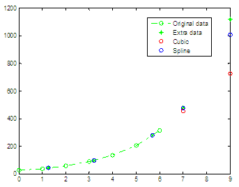
inter/extrapolate with 'spline' method produces
this plot  we can
see that interpolations work pretty well, but extrapolations diverge
from the
expected results. We can see that a spline method works better than a
cubic one
in this case, just for extrapolations. From 'Exponential Regression' to 'Matlab Programming'
|


