High-Pass
Filter Simulator
(WinSpice and Scilab interface)
In this article we present a Scilab routine to drive the simplest
high-pass filter designed in the WinSpice simulator. This method can
also be
easily adapted to simulate and drive any circuit entered in SPICE.
SPICE stands
for Simulation Program with Integrated Circuit Emphasis.
The
concept of the Scilab driver is illustrated by
simulating a very simple RC high-pass filter. In this example
we're using specifically
Scicoslab ver. 4.3 (Scilab compatible) and WinSpice3 ver. 1.04.07.
For more information about Scicoslab, visit scicoslab.org.
For more information about WinSpice, visit www.winspice.com.
Interchanging information between Scilab and WinSpice allows
the
implementation of optimization techniques and graphical
possibilities not
included in the simulator environment itself. The shown approach is
very
flexible and utilizes the inherent capability of this SPICE
simulator to
include text files with parameters and print data to external
.csv (comma separated values) files.
This is the general
idea... - First, the
circuit in Spice is designed and defined (.cir file). This
circuit is simulated and tested within the WinSpice
environment before any
attempt is made to interact with Scilab. We separate the parameters or
components
of interest and include them in another text file (using the .include
directive
in the main file).
-
Second, we write the output of the simulator to an external file, that
is, we
include 'write' commands in the main .cir file so that the
results are
saved as external (.csv) text files that can be read by Scilab.
-
Third, now we just have to write parameters, run the simulation and
read the
response. All this can be done from/by Scilab as if the simulator was
an
ordinary built-in function to be called!
Now, let's see the details with a specific example...
First
Step
We create, test
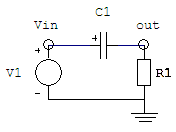
and simulate this simple RC high-pass filter in WinSpice:

We initially (arbitrarily) use these values:
R = 10k ohms, C = 1 nF
The main .cir file (which is also a text file) is:
---- RC
- High Pass Filter ----
V1 Vin 0
dc
0 ac 1
.include param_hpf.txt
R out 0 {res1}
C vin out {cap1}
.control
AC DEC
10 10 1MEGHZ
plot
vdb(out)
.endc
.end
The actual parameters are
located in a separate file named ‘param_hpf.txt’,
which in this case contains one line only:
.param
res1= 1.000000e+004 cap1= 1.000000e-009
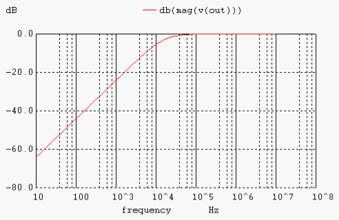
As expected, the frequency analysis delivers this result:

Second Step
We include appropriate 'write' commands in the main .cir file, so that
the
results are saved as .csv files available to Scilab. The 'quit' command allows us to close the simulator window.
The control block changes into:
.control
AC DEC
10 10 10MEGHZ
plot
vdb(out)
write
RC_HPF_ac_out.csv vdb(out)
quit
.endc
Third Step
We now create a function to be run by Scilab to write the text
file that includes
the parameters, launch the simulator and read the results. This is
the code to accomplish it:
function [x, y] = WS_high_pass_filter(p)
// Create and save the file 'param_hpf.txt' to be included
in
// the circuit to be run by WinSpice.
[fd, err] = mopen('param_hpf.txt', 'w');
n = mfprintf(fd, "%s %e %s %e \n", '.param res1=',
p(1), 'cap1=', p(2))
mclose(fd);
// Run WinSpice
// Make sure wspice3.exe and all the involved files are
available
// in this directory
host('wspice3 high_pass_filter.cir')
// Read data saved in the
.csv file
[x, y] =
getWSpicedata('RC_HPF_ac_out.csv');
endfunction
There is an important portion of additional code to
read the .csv files.
function [x, y] = getWSpicedata(f);
// f = name of the .csv file
// x = frequencies
// y = response of the circuit in dB
// We open the file and discard the first
row
[fd, err] = mopen(f, 'r');
s = mgetl(fd, 1);
// We start reading all the
rows, we read them as strings
// We
keep on reading until we reach an empty row
ix = 1;
while
~meof(fd)
s = mgetl(fd, 1);
if s == []
break
end
// 'strindex' finds
the position of all the commas in the string
k = strindex(s,
',');
// 'part' extract a
portion of the string
// 'eval' converts
the string into a number
// we take only the
first and the third columns
x(ix) = eval(
part(s, 1 : k(1)-1) );
y(ix) = eval(
part(s, k(2)+1 : k(3)-1) );
ix = ix + 1;
end
mclose(fd);
endfunction
Now, we're ready to perform some
simulations driving
WinSpice from Scilab.
xdel(winsid()); clear; clc
// We declare our functions to drive the
circuit
getf('WS_high_pass_filter.sci')
getf('getWSpicedata.sci')
// We decide our parameters
p = [10e3 1e-9];
// This function calls WinSpice and reads
the results
[x y] = WS_high_pass_filter(p);
// We now plot the response of the circuit
plot2d(x, y, logflag="ln")
xgrid
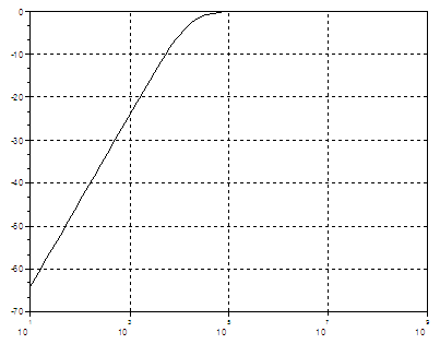
For R1 = 10k ohms and C1
= 1 nF, we get this AC response in
dB.

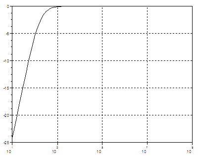
For R1 = 1k ohms and C1 =
1 uF, we run it like this...
p = [1e3 1e-6];
[x y] =
WS_high_pass_filter(p);
This is the new AC response in dB:

We
can now use WinSpice as if it was another Scilab or Scicoslab
function! This means that we can work through circuit optimization
using
functions such as leastsq, datafit, optim, and others.
The main idea is that now we can try some numbers in our design, we can
simulate the results and use Scilab to modify relevant
values in the
circuits, iteratively in optimization routines. Maybe you'd like to see a similar example on a low-pass filter in Matlab.
Reference:
http://www.desi.iteso.mx/erayas/cad.htm, 2012.
From
'High Pass Filter' to home
From
'High Pass Filter' to Scilab examples


|


