Lagrange Interpolation
(curvilinear
interpolation)
The computations in this
small article show the Lagrange
interpolation. The code computes y-coordinates
of points on a curve given their x-coordinates.
You must enter coordinates of known
points on the curve, no two having
the same
abscissa.
This is the simple
function:
function y0 =
lagrange_interp(x, y, x0)
%
x is the vector of abscissas.
%
y is the matching vector of ordinates.
%
x0 represents the target to be interpolated
%
y0 represents the solution from the Lagrange interpolation
y0 = 0;
n =
length(x);
for j = 1 :
n
t
= 1;
for i = 1 : n
if i~=j
t = t * (x0-x(i))/(x(j)-x(i));
end
end
y0 = y0 + t*y(j);
end
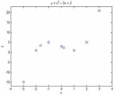
Example 1 - Interpolate a cubic function
Consider the curve y
= x3 - 3x + 3. We now that points
x = [-3
-2 -1 0 1 2 3];
y = [-15
1 5 3 1 5 21];
are
on the curve. What are the
values of y when x
= -1.65 and 0.2?
x1 =
-1.65;
y1 =
lagrange_interp(x,y,x1)
x2 = .2;
y2 =
lagrange_interp(x,y,x2)
The
results are:
y1 =
3.4579
y2 =
2.4080
Let’s
plot our approach:
plot(x,
y, 'bo', x1, y1, 'ro', x2, y2, 'ro')
axis([-4
4 -17 23])
title(‘y = x^3 – 3x + 3’)
xlabel(‘x’)
ylabel(‘y’)
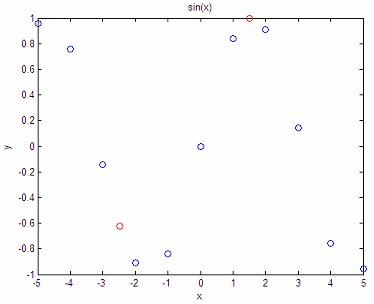
Example 2 - Interpolate a
sine function
Given the following
points from a sine curve, what are the y-values
for x = -2,47 and x
= 1.5?
x = [-5
-4 -3 -2 -1 0 1 2 3 4 5];
y =
[.958 .757 -.141 -.909 -.841 0 .841 .909 .141 -.757 -.959];
x3 =
-2.47;
y3 =
lagrange_interp(x,y,x3)
x4 =
1.5;
y4 =
lagrange_interp(x,y,x4)
The
results are:
y3 = -0.6218
y4 = 0.9972
And our plot is:
plot (x,
y, 'bo', x3, y3, 'ro', x4, y4, 'ro')
title('sin(x)')
xlabel('x')
ylabel('y')
The approximation is not bad, right? In fact, it seems to be quite
accurate!
From
Lagrange
Interpolation to home
From
Lagrange Interpolation to Generic Programming


|


