
Least Squares FitCurve Fit in Scilab / Scicoslab
The
goal of this article is to provide a simple demonstration of the use of
the ‘leastsq’
function in Scilab, which is used to solve nonlinear least squares
problems. Let’s
say that initially we have some measured data points and that we know
the form
of the function that we should be getting, but we don’t know the
coefficients
involved. We can develop a simple and practical approach for the fit
using the
least squares fit function provided in Scilab. Without a rigorous mathematical view, the ‘leastsq’ function minimizes with respect to x the function:  which
is the sum of the squares of the components of fun. Bound
constraints
may be
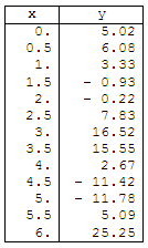
imposed on x. Let’s suppose
that this is our measured information. 
We can
create a file named 'nonlinear_fit_1.sci'
with the following two
functions, one
(fun2fit) to calculate the function and another (myerror) to work
on the
error to be reduced: //
This
is the function to be approximated. //
This
is how we define the error to be minimized. Now, we
are going to develop the main script which is going to launch the
optimization
function. //
Delete figures, memory and screen //
Declare the objective function, or function to be minimized //
Define our initial data or measured points //
This
is our guessed coefficients. First attempt. //
Plot
the original points and the starting point in our problem //
Launch the optimization function. Provide data and coefficients //
Plot
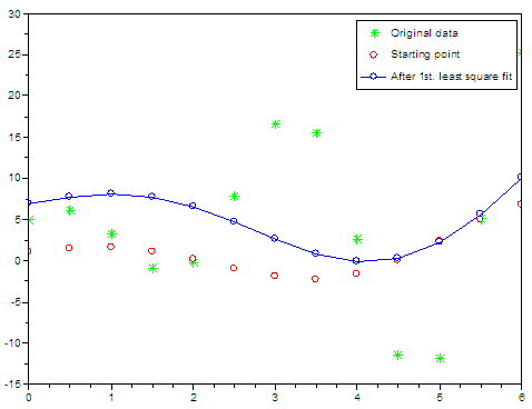
results after optimization This is
the comparison of the different situations in our problem.
The
solution provided by the least-squares fit is copt = f
= The
function result (f) is a very large number. It should be as close to
zero as
possible.
//
This
is our guessed coefficients. Second attempt. set("current_figure",
1) [f,
copt] = leastsq(list(myerror, x, y), c0) This is
the comparison of the different situations in our problem, in our
second
experiment.
The new
results are: copt = f
=
The
function is close enough to zero and now the solution is what we
needed. We have found the coefficients in our problem. From 'Least Squares Fit' to Matlab home From 'Least Squares Fit' to Scilab examples
|


