Maclaurin series - some mathematical experiments with Matlab

If you’re approximating a function value for an x-value far from 0, you’ll have to use the slightly more complicated Taylor series, which work almost exactly like Maclaurin series, except that you can center them at any x-value.
 

Mathematically, we say the Maclaurin series approximates values of f(x)
very accurately, as long as those x-values are close to 0.
 

When you work with these sequences, you’ll actually be generating Maclaurin polynomials, which are some finite terms of the series. Before you start generating the terms to be added, make sure you understand the formula.

In case you don’t know what f⁽ⁿ⁾(0) means, it is the n^th derivative of f(x)  evaluated at 0. For example, f⁽⁴⁾(0) is the fourth derivative of f(x) with x = 0.
 

The Maclaurin series generates good approximations of f(x), as long as
x is close to 0. You won’t use an infinite series to calculate the approximation. The more terms you use, however, the better your approximation will be.
 

As an example, let’s use the Maclaurin polynomial (with just four terms in the series) for the function f(x) = sin(x) to approximate sin(0.1).
 

We first write the terms of the series from n = 0 to n = 3.
 

 
And we’ll need to take four derivatives of the function and then evaluate them at x = 0.
 

Definition 1: f⁽⁰⁾(x) is the function itself. There’s no derivative.
Definition 2: 0! = 1. 

f⁽⁰⁾(x) = sin(x)   f⁽⁰⁾(0) = sin(0) = 0
f⁽¹⁾(x) = cos(x)   f⁽¹⁾(0) = cos(0) = 1
f⁽²⁾(x) = -sin(x)  f⁽²⁾(0) = -sin(0) = 0
f⁽³⁾(x) = -cos(x)  f⁽³⁾(0) = -cos(0) = -1 


Let’s create a script in Matlab to evaluate the series just with 4 terms (0 to 3):
 

clear, clc 

% Let's see more decimals
format long 

% We go from n = 0 to n = 3
n = 0 : 3; 

% This is the point for evaluation
x = 0.1; 

% These are the derivatives for each term
d = [0 1 0 -1]; 

% We form the sequence, following the formula
seq = d .* x.^n ./(factorial(n)) 

% We add-up to get the Maclaurin approximation
approx = sum(seq) 

% Let's compare with the official number
real_value = sin(x)

The response is:
 

seq = 0    0.10000000000000    0  -0.00016666666667
approx =       0.09983333333333
real_value =   0.09983341664683

We’ve got almost the exact value by using only 4 terms of the series (and two values are zero, because the derivative is zero for those terms). If we had used n = 8, it would have been an even better approximation.
 

Now, let’s develop (code) an automated series to express the sine function (centered at 0) using the Maclaurin expansion and let’s compare the results with different number of terms included.

function smp = maclaurin_sin(x, n)
% x = a vector with values around 0
% n = number of terms in the series 

% Start the series with 0
smp = 0;

% Consider all the possible derivatives
deriv = [0 1 0 -1]'; 

% Iterate n times (from 0 to n-1)
for i = 0 : n-1

    % Implement the Maclaurin expansion
    t(i+1, :) = deriv(1) * x.^(i) / factorial(i);

    % Find the derivative for the next term
    deriv = circshift(deriv, -1);

end

% Add-up the calculated terms
smp = sum(t);    

Note: the above code is not very efficient, because we’re calculating and adding terms even when their derivative is zero, which is a waste of 50% of the time, more or less. We’ll leave it as-is just to keep and show the natural flow of the formula... 

Now, let’s create a script to test and use the function above. 

clear, clc, close all 

% Work with two full periods
x = -2*pi : .1 : 2*pi;
y = sin(x); 

% Plot the goal
plot(x, y, 'g', 'Linewidth', 3)
title('Study of Maclaurin series')
xlabel('x')
ylabel('sin(x) with different number of terms')
axis([-2*pi 2*pi -3 3])
grid on
hold on 

% Consider 4 terms
smp = maclaurin_sin(x, 4);
plot(x, smp, 'ro') 

% Consider 6 terms
smp = maclaurin_sin(x, 6);
plot(x, smp, 'b-.') 

% Consider 10 terms
smp = maclaurin_sin(x, 10);
plot(x, smp, 'k', 'linewidth', 3) 

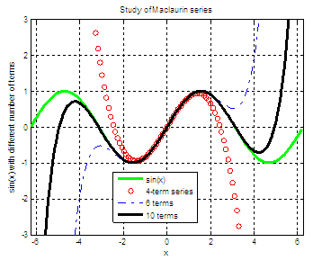
% Label the calculated lines
legend('sin(x)', '4-term series', ...
       '6 terms', '10 terms') 

The results are:

 
We see that all of the expansions work well when we are close to 0. More terms approximate better a larger portion of the sine curve.