Mathematical
Optimization
|
Matlab
includes at least two standard functions intended for numerical
or mathematical
optimization. These instructions are ‘fminbnd’ (for one
single variable) and ‘fminsearch’
(for one or more variables).
Built-in function ‘fminbnd’
tries to find a minimum of a function of one variable within a fixed
interval.
|
Built-in function ‘fminsearch’
finds the minimum of a scalar function of several variables, starting
at an initial estimate. This can be also considered as unconstrained
nonlinear optimization. Both functions obtain a local minimum, not a
global one.
Since we can explore and express a function in terms of a predefined
error, minimizing this error function equals optimizing the function.
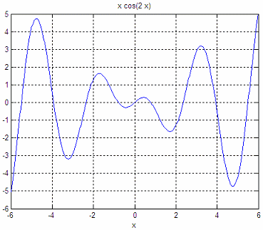
Let’s work with this expression:
It can be
defined in this way:
function y =
xcos2(x)
y =
x*cos(2*x);
and it
can be easily plotted like this:
ezplot('x*cos(2*x)')
axis([-6
6 -6 5])
grid on

We
can implement a minimization method in the range [-5, 0],
like this (the fminbnd algorithm is based on golden section
search and
parabolic
interpolation):
options
= optimset('Display','iter','TolX',0.001);
[xc,
FunVal, EF, output] = fminbnd(‘xcos2’, -5, 0, options)
Matlab displays the
following answer. We get the number of
times that the function was evaluated, the point of evaluation and the
function
value at each iterate.
Func-count x
f(x)
Procedure
1
-3.09017
-3.07384
initial
2
-1.90983
1.48735
golden
3
-3.81966
-0.813651
golden
4
-3.02998
-2.95481
parabolic
5
-3.21391
-3.18035
parabolic
6
-3.22291
-3.18038
parabolic
7
-3.21865
-3.1805
parabolic
8 -3.21832 -3.1805
parabolic
9
-3.21899
-3.1805
parabolic
Optimization terminated:
the current x
satisfies the termination criteria using OPTIONS.TolX of 1.000000e-003
xc = -3.2187
FunVal = -3.1805
EF = 1
output =
iterations: 8
funcCount: 9
algorithm:
'golden section search, parabolic interpolation'
message: [1x112
char]
The value xc = -3.2187 is the best value found after our mathematical
optimization. If we change the ‘TolX’
parameter of the options included in
the optimization function (fminbnd), we get a different amount of
function
evaluations
and, naturally, a slightly different minimum value. We must be aware
that
changes in tolerances naturally affect our results.
options
= optimset('Display','iter','TolX',0.1);
Func-count
x
f(x)
Procedure
1
-3.09017
-3.07384
initial
2
-1.90983
1.48735
golden
3
-3.81966
-0.813651
golden
4
-3.02998
-2.95481
parabolic
5
-3.21391
-3.18035
parabolic
6 -3.24725
-3.17502
parabolic
7
-3.18058
-3.17092
parabolic
Optimization terminated:
the current x
satisfies the termination criteria using OPTIONS.TolX of 1.000000e-001
xc = -3.2139
FunVal = -3.1804
EF = 1
output =
iterations:
6
funcCount: 7
algorithm:
'golden section search, parabolic interpolation'
message: [1x112
char]
If
we now change the range of exploration to [0, 6], we find
another minimum:
Func-count
x
f(x)
Procedure
1
3.81966
0.813651
initial
2
6.18034
6.05006
golden
3
2.36068
0.0211764
golden
4
2.47085
0.561649
parabolic
5
1.45898
-1.42265
golden
6
1.66467
-1.63542
parabolic
7
1.69841
-1.64339
parabolic
8
1.73174
-1.6428
parabolic
Optimization terminated:
the current x
satisfies the termination criteria using OPTIONS.TolX of 1.000000e-001
xc = 1.6984
FunVal = -1.6434
EF = 1
output =
iterations:
7
funcCount: 8
algorithm:
'golden section search, parabolic interpolation'
message: [1x112
char]
Now, let’s explore the
same function with fminsearch.
We’re
going to run different
starting points, with this code:
fun = 'xcos2';
options
= optimset('Display','iter','TolX',0.1);
i = 1;
for sx = -5
: .1 : 5
[xc,
FunVal, EF, output] = fminsearch(fun,
sx, options);
x(i)
= sx;
xo(i)
= xc;
oi(i)
= output.iterations;
of(i)
= output.funcCount;
i
= i+1;
end
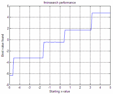
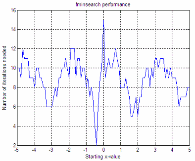
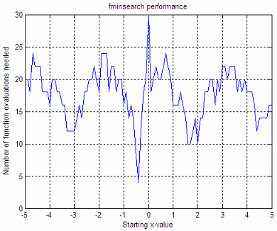
We get these graphics:
These graphics say that
if we start with x = -3, the minimum
found after our mathematical optimization is y = -3.22, it takes 6
iterations to reach that value, and 12
function
evaluations are needed to reach that minimum. If we start with x = 4,
the
minimum found is 4.8, it takes 9 iterations, and 18 function
evaluations to
reach that minimum.
We must be very aware
that different initial
conditions and
tolerances lead us to different results. Mathematical
optimization is not
straigthforward most of the times.
From
'Mathematical Optimization' to home
From
'Mathematical Optimization' to Matlab Programming


|


