Nodal Analysis - KCL and Matlab

 
In this type of analysis, if there are n nodes in a circuit, and we select a reference node (node 0), the other nodes can be numbered from V₁ through V_n-1.

With one node selected as node 0 (reference), there will be n-1 independent equations. If we assume that the admittance between nodes i and j is given as Y_ij, we can write the following equations including all of the nodes in the circuit: 

 
where: 

m = n - 1
V₁, V₂,..., V_m are voltages from all the nodes with respect to node 0

 is the algebraic sum of current sources at node m.

 
The above system of equations can be expressed in matrix form as: 

Y V = I
 

And naturally, its solution is: 

V = Y ^-1I, which in Matlab can be easily solved using the backslash operator (\), like this: 

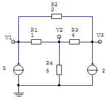
V = Y\I

The following example illustrates the use of Matlab for solving nodal voltages of electrical circuits. 

Nodal Analysis - find the voltages in a circuit

For the circuit shown below, resistors are in ohms and current sources are in amps. We’re asked to find the nodal voltages V₁, V₂, and V₃.

Using KCL, and forming our matrices Y and I, let’s see...

For node V₁ we have,  

and the first row of our Y matrix is going to be the coefficients for the voltages. This means that we can form our matrix in Matlab like this: 

Y(1,:) = [(1/1 + 1/2)  -1/1  -1/2];
and naturally I(1) = 5;

At node V₂,  

the second row of our Y matrix is going to be the new set of coefficients for the voltages. Letting Matlab work out the operations, we express

Y(2,:) = [1/1  (-1/1 - 1/4 - 1/5)  1/4];
and I(2) = 0;

Finally, at node V₃ we have,   

thus, our third row of the Y matrix is 

Y(3,:) = [-1/2 -1/4 (1/2 + 1/4)];
and I(3) = 2;

Summarizing our findings, we fill-in our matrices Y and I, like this:

Y = 1.5  -1.00   -0.50
    1.0  -1.45    0.25
   -0.5  -0.25    0.75 

I =  5
     0
     2
 

The solution is easy using Matlab: just type V = Y\I. The answer is matrix V, with three rows (our vector of unknowns contains three variables in a column: V₁, V₂ and V₃)

 
V = 40.4286
    35.0000
    41.2857