Normal Distribution

This algorithm (program in Matlab) calculates the probability and frequency of given values on a standard normal distribution curve (Gauss’ bell). 

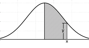
Standard Normal distribution

The shaded area represents the probability of ‘x’, and its frequency is ‘y’.
The normal probability is approximated using the following formula: 

where:
                             a₁ = 0.4361836
                             a₂ = -0.1201676
                             a₃ = 0.9372980
                             
                             t = 1/(1 + 0.33267x)
                             eps < 10^-5

 This is the Matlab code to accomplish the task,

 % Clears screen and deletes all the variables in the workspace
clc; clear; 

% Asks the user for input
m = input('Mean: ');
s = input('Std. Dev: ');
y = input('x = '); 

% Calculates the frequency (y coordinate)
y = abs((y - m)/s);
r = exp(-y^2/2)/sqrt(2*pi);
str = ['Frequency: ' num2str(r)];
disp(str) 

z = y;
% Approximates probability (area under curve)
y = 1/(1 + 0.33267*abs(y));
a1 = 0.4361836;
a2 = -0.1201676;
a3 = 0.9372980;
t = 1 - r*(a1*y + a2*y^2 + a3*y^3);
if z < 0
    t = 1 - t;
end

str = ['Probability: ' num2str(t)];
disp(str)

Example 1:

The mean instructions per millisecond (IPMS) of a certain type of modern computers is 150. The standard deviation is 15 IPMS. If the IPMS are normally distributed, what is the probability that a computer executes between 150 and 180 instructions per millisecond?

Easy. Run the Matlab code above and enter...

Mean: 150
Std. Dev: 15
x = 180 

The handy Matlab response is 

Frequency: 0.053991
Probability: 0.97724

Example 2: 

What if we need to know the probability of an execution of 130 and 150 instructions per milliseconds for the same type of modern computers?

Don’t worry, Matlab is here... 

Mean: 150
Std. Dev: 15
x = 130

Again, the handy response is 

Frequency: 0.16401
Probability: 0.9088

 From 'Normal Distribution' to home

 From 'Normal Distribution to 'Probability and Statistics' Menu