Piecewise function - separate ranges in Matlab

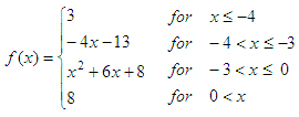
We’re going to experiment in Matlab with this type of functions. We’re going to develop three ways to define and graph them. The first method involves if-statements to classify element-by-element, in a vector. The second method uses switch-case statements, and the third method uses indices to define different sections of the domain.

Let’s say that this is our piecewise-defined function  

 

and we’d like to graph it on the domain of -8 ≤ x ≤ 4

Method 1. If-else statements

First, let define our function with if-else statements. We just use different conditions for the different ranges, and assign appropriate values.

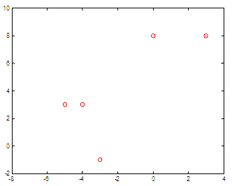
function y = piecewise1(x)
if x <= -4
    y = 3;
elseif -4 < x & x <= -3
    y = -4*x - 13;
elseif -3 < x & x <= 0
    y = x^2 + 6*x + 8;
else
    y = 8;
end

Now, we can use scalars or arrays to call this function, in a classical way:

% Define elements
x = [-5 -4 -3 0 3]
% Submit element-by-element to the function
for ix = 1 : length(x)
    y(ix) = piecewise1(x(ix))
end
% Plot discrete values
plot(x, y, 'ro')
% Define x and y ranges to display
axis([-8 4 -2 10])
 

The result is:

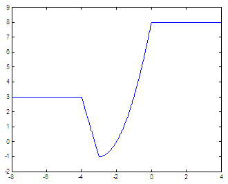
Let’s say that we need more values. We can call our function this way

x = -8 : .01 : 4;
for ix = 1 : length(x)
    y(ix) = piecewise1(x(ix));
end
plot(x, y)
axis([-8 4 -2 9])
 

The new graph (which obviously gives more information) is:

 

Method 2. Switch-case statements

Our second method classifies the elements using switch-case statements. We separate the different ranges in different cases. If that condition is true, then the switch-expression will match the case-expression, and the appropriate statements will be executed.

function  y = piecewise2(x)
switch x
    % A scalar switch_expr matches a case_expr if
    % switch_expr == case_expr
    % The first case must cover the x = 0 case
    case x * (-3 < x & x <= 0)
        y = x^2 + 6*x + 8;
    case x * (x <= -4)
        y = 3;
    case x * (-4 < x & x <= -3)
        y = -4*x - 13;
    otherwise
        y = 8;
end

One important note is that when x = 0 the result of the case-expression is also 0, and the first case executes. That’s why we need to place our x = 0 case first in the structure, otherwise we get wrong that point.

We can test our second piecewise function definition, like this: 

x = -8 : .01 : 4;
for ix = 1 : length(x)
    y(ix) = piecewise2(x(ix));
end
plot(x, y)
axis([-8 4 -2 9]) 

and get the previous graph, too.
 

Method 3. Vectorized way

The above routines assume that we’re entering scalars as input parameters. Now, we’ll assume that we’re submitting whole vectors, and we’ll handle indices for that.

A very useful instruction for this is the Matlab built-in function ‘find’. 

This line x2 = x(-4 < x & x <= -3);
assigns to x2 the values of matrix x that meet the criteria -4 < x ≤ -3
 

The line find(-4 < x & x <= -3)
finds just the indices (not values) of matrix x that meet the same criteria.
 

We can combine those two ideas to work out the appropriate values for that range. 

The following code is just one way to take full vectors and pack them into piecewise functions:

function  y = piecewise3(x)
% first range
y(find(x <= -4)) = 3; 

% second range
x2 = x(-4 < x & x <= -3);
y(find(-4 < x & x <= -3)) = -4*x2 - 13; 

% third range
x3 = x(-3 < x & x <= 0);
y(find(-3 < x & x <= 0)) = x3.^2 + 6*x3 + 8; 

% fourth range
y(find(0 < x)) = 8;
 

Now, we can avoid for-loops before graphing this type of functions...
We enter the whole array (independent variable values) as parameter

x = -8 : .01 : 4;
y1 = piecewise3(x);
plot(x, y1)
axis([-8 4 -2 9])

this produces what we know and expect...