Polynomial Regression – Least Square Fittings

p is a row vector of length n + 1 containing the polynomial coefficients in descending powers, p(1)*x^n + p(2)*x^(n - 1) + ... + p(n)*x + p(n + 1).

y = polyval(p, x) returns the value of a polynomial p evaluated at x. p is a vector of length n + 1 whose elements are the coefficients of the polynomial in descending powers, y = p(1)*x^n + p(2)*x^(n - 1) + ... + p(n)*x + p(n + 1). If x is a matrix or vector, the polynomial is evaluated at all points in x.

Let’s say that we’re given these points 

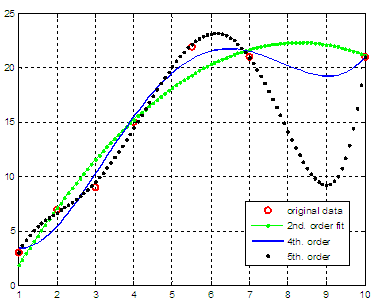
x = [1 2 3 4 5.5 7 10]
y = [3 7 9 15 22 21 21] 

and want to explore fits of 2nd., 4th. and 5th. order. We could use the following code:
 

clear all, clc, close all, format compact

% define coordinates
x = [1 2 3 4 5.5 7 10];
y = [3 7 9 15 22 21 21];

% plot given data in red
plot(x, y, 'ro', 'linewidth', 2)
hold on 

% find polynomial fits of different orders
p2 = polyfit(x, y, 2)
p4 = polyfit(x, y, 4)
p5 = polyfit(x, y, 5) 

% see interpolated values of fits
xc = 1 : .1 : 10; 

% plot 2nd order polynomial
y2 = polyval(p2, xc);
plot(xc, y2, 'g.-') 

% plot 4th order polynomial
y4 = polyval(p4, xc);
plot(xc, y4, 'linewidth', 2) 

% plot 5th order polynomial
y5 = polyval(p5, xc);
plot(xc, y5, 'k.', 'linewidth', 2)
grid

legend('original data', '2nd. order fit', '4th. order', '5th. order')

The resulting fits are displayed in this figure

The coefficients found by Matlab are:

p2 =    -0.3863    6.3983   -4.1596
p4 =     0.0334   -0.7377    5.0158   -8.4137    7.5779
p5 =     0.0213   -0.5022    4.1330  -14.5708   25.3233  -11.3510

 
which, in other words, represent the following polynomials of  2nd., 4th. and 5th. order, respectively.

 
y₂ = -0.3863x² + 6.3983x - 4.1596
y₄ =  0.0334x⁴ - 0.7377x³ + 5.0158x² - 8.4137x + 7.5779
y₅ =  0.0213x⁵ - 0.5022x⁴ + 4.1330x³ - 14.5708x² + 25.3233x - 11.3510