
RC CircuitTransient Analysis with MatlabConsidering the RC
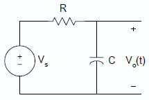
Circuit (also called RC network) shown in
this figure
we can use the
Kirchhoff’s current law (KCL) to write the
following equation
and we can
rearrange into the equation
 The solution to the
equation above is  where This solution represents
the voltage across a discharging
capacitor. Now, to obtain the
voltage across a charging capacitor, let
us consider this figure that includes a voltage source   If the capacitor is not
charged initially, that is v0(t)
= 0 when t = 0, then the solution to the equation above is given by 
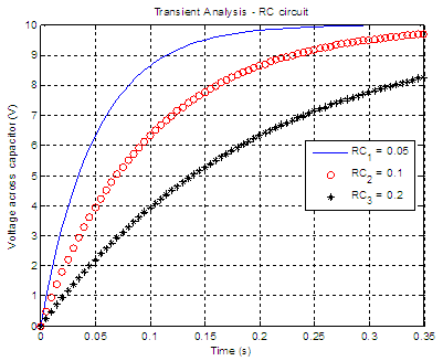
Example 1 – Charging circuit
Assume that for the
charging RC circuit above Vs = 10 volts
and C = 10 microfarads. Plot the voltage across the capacitor if R
equals 5k ohm,
10k ohms and 20k ohms. This just means that we are going to explore
three time
constants. This code is one simple
solution to the problem %
Define the voltage source %
Define the resistors in each time constant and R2 =
10e3; R3 =
20e3; %
Plot the responses, all at once
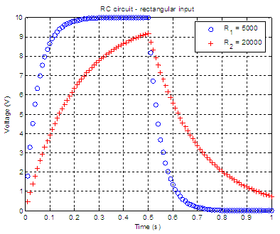
Example 2 -
Charging
/ discharging RC circuit
In the same charging
circuit above, the input voltage is now
a rectangular pulse with an amplitude of 10 volts and a width of 0.5
seconds. If
C = 10 microfarads, we’ll plot the output voltage, v0(t),
for a resistance R equal to 5k ohms, and 20k ohms. The plots
should start from 0s and end at 1s. We are going to develop a function that will return the voltage and corresponding time of the response. We need to use the two formulas mentioned previously and that’s why we separate our code in two halves. The input parameters are
the voltage source (vs), the
resistor (r) and capacitor (c). function [v, t]
= rectangular_RC(vs, r, c) %
First half of the pulse: 0.01 to 0.5 seconds %
Second half of the pulse: 0.51 to 1 seconds. t = [t1 t2]; v = [v1 v2]; Now, we are going to call
the function from our main code,
like this %
Given constants %
Case 1. R = 5k ohms %
Case 2. R = 20k ohms %
Plot the responses %
Add labels
From 'RC circuit' to Matlab home From 'RC circuit' to Electrical Calculations
|


