Heaviside Unit Step Function

The function depends on real input parameters. We can define the function having a scalar number as an input. For example, let’s create a discrete plot without using any special toolbox in Matlab.

function y = step_fun(n)
% We assume a scalar input
% Our default output value is 0
y = 0; 

% We change our output to 1 if the argument is greater 
% than or equal to 0
if n >= 0
    y = 1;
end

If we want to get a plot from there, we have to iterate utilizing real numbers. If the input is an integer, then the function will be a discrete one. To stress the fact that we're working with discrete functions here, we'll use 'stem' instead of 'plot'.

Let's call the function from another script. For example: 

% We iterate from -5 to 5 using only integers
for n = -5 : 5
    y = step_fun(n);
    stem(n, y)
    hold on
end
% We adjust our axis values just to visualize better
axis([-5 5 -1 2])

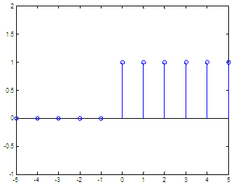
and we get

Now, let’s say that we have a vector (not a scalar) as an input. We want to calculate the Heaviside function for all of the values included in the vector. We can create another function to considerate this approach:
 

function y = heaviside(n)
% We assume a vector input 

% Our default output value is 0
y = 0 * n;
% Now, we find values in n greater than or equal to 0
y(find(n >= 0)) = 1;

 
We don’t need a loop now, so our process has been simplified a lot. Let's use this new approach.

n = -5 : 5;
y = heaviside(n);
stem(n, y)
axis([-5 5 -1 2])

 
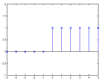
The result is again: 

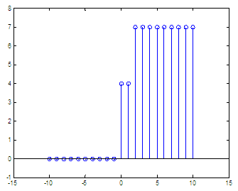
If we want to calculate y = 4H(n) + 3H(n-2), in a range of integers that go from -10 to 10, we can do simply this: 

n = -10 : 10;
y = 4 * heaviside(n) + 3*heaviside(n-2);
stem(n, y)
axis([-15 15 -1 8])  

and the result is:

 

We can see that every integer in the domain of the function counts to add to the final result, and that happens when the argument is zero for each term. The first term, 4H(n), adds a height of 4 (coefficient) at n = 0; the second term, 3H(n-2), adds a magnitude of 3 at n = 2.