Learn to solve definite
integrals with a numerical software
How
to
calculate integrals with Matlab
|
In computerized
or numerical methods, a numerical integration can be performed by a
number of
algorithms that calculate the approximate value of definite integrals.
Numerical
evaluation of the integral  is
called quadrature. The
term ‘numerical quadrature’ is more or less a synonym for numerical
integration, especially if applied to one-dimensional integrals. is
called quadrature. The
term ‘numerical quadrature’ is more or less a synonym for numerical
integration, especially if applied to one-dimensional integrals. |
We’re
going to focus this time on the calculation of definite integrals using
the
Matlab already built-in functions.
Why
we
can evaluate definite integrals
There’s
a number of reasons for carrying out numerical integration. The
integrand f(x)
may be known only at certain points, such as obtained by sampling. Some
digital
systems and other computer applications may need integral calculus for
this
reason.
A
formula for the integrand could be known, but it may be difficult or
impossible
to find an analytical integral.
It may
be possible to find an antiderivative, but it may be easier to compute
a
numerical approximation. That may be the case if the exact integral is
given as
an infinite series, or if its evaluation requires a special function
which is
not available.
Matlab
provides the following built-in functions for numerical integration:
quad
- Uses
adaptive Simpson quadrature.
Basic
form: q = quad(FUN, A, B), which tries to approximate the integral of
scalar-valued function FUN from A to B to within an error of 1 x 10⁻⁶
using recursive adaptive Simpson quadrature. The function Y = f(X) should accept a vector argument X and return a vector result Y, the integrand evaluated at each
element of X.
quadl
–
Uses adaptive Lobatto quadrature.
Basic
form: q = quadl(FUN, A, B), which tries to approximate the integral
using high
order recursive adaptive quadrature.
Let’s
work on some examples and learn a little bit about intgral calculus...
Single
integration
The
Gaussian integral (aka Euler-Poisson integral or Poisson integral) is
the
integral of the Gaussian function over the entire real numbers.

Since
the result is exact for a known interval, let’s use this function as a
guinea
pig.
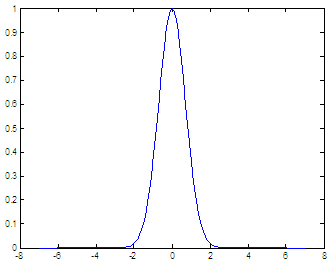
First,
let’s plot it to see what we’re doing. We cannot go from -infinity to
infinity,
but we can use a more reasonable interval.
x = -7 :
.1 : 7;
y =
exp(-x.^2);
plot(x,
y)
and we
get
Now, we
see that if we integrate in the interval [-8, 8] we can get a very good
answer.
We don’t have to go beyond that.
You can
define a separate function for the integrand, and use its name within
the quad
function. In this case, the expression is simple and we’re going to use
it
directly as an argument to the quadrature
format long
y1
=
quad('exp(-x.^2)', -8, 8)
y2 =
quad('exp(-x.^2)', -20, 20)
and the
answers are
y1
= 1.77245489096641
y2 =
1.77245399494936
Obviously,
the second answer is better than the first one (according to sqrt(pi)), due to the longer interval,
but
even the first answer is correct to 5 digits.
You can
type help quad
or help quadl
on your Matlab command window to see a full description
of the usage and examples of the functions.
Double
integration
To
evaluate definite integrals of the form
there’s
the function dblquad. The basic syntax for double integration is:
II =
dblquad(‘fxy_fun’, x_min, x_max, y_min, y_max)
Let’s
compute the following double integral
f =
inline('x.^2
+ 4*y');
ii =
dblquad(f, 11, 14, 7, 10)
and the
result is 1719
From
'Definite Integrals'
to home
From
'Definite
Integrals' to 'Calculus Problems'


|


