Find
Intersections - an engineering approach
The
problem of how to find
intersections of given lines is
very common in math or basic algebra.
The meaning of those intersections is
that the given lines or curves have the same coordinate values
at some points.
In other words, those lines or functions have simultaneously the same x and y
(or even z)
values at those points called intersections.
This also means that
if we divide the y-value
of one function by the y-value
of the other function,
we’re going to get 1 at the intersection point.
Also, if we subtract
the
y-value
of the first function from the y-value
of the second function at the
intersection point, we’re going to get 0.
You can find in this site
some articles on how to solve
linear
systems or nonlinear
systems, from a more numerical point of view.
In this article, we’re
going to develop a basic an practical
approach using a different technique, naturally employing the available
Matlab
resources. We’re also going to become aware of inherent inaccuracies of digital
systems.
Let’s say that we have functions
y1
= x + 3 (a
straight line) and
y2
= x2
– 4 (a parabola)
and we want to find their
intersections.
First approach. Visualize the functions.
We can get points from
those functions and plot them, like this:
x = -4 :
.1 : 4;
y1 = x +
3;
y2 =
x.^2 -4;
plot(x,y1,'b', x,y2,'r')
grid on
title('Intersection')
xlabel('x')
ylabel('y')
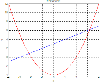
The Matlab figure is:

and now we can easily
understand how the lines behave and
where the intersections are. We can zoom-in the image if needed (use
the appropriate icon on the figure menu).
Second approach. Divide element-by-element.
If
we need a numerical result and want to find intersections, we can
divide one function by the
other (element-by-element), and when we get a 1 we know that we’ve
found an
intersection point. On the practical side, however, we must be aware
that our
lines are not continuous. We defined x in steps of 0.1
(above). We see
a continuous
line because Matlab is plotting that, but our vectors are not really
continuous (that’s not possible with digital computers).
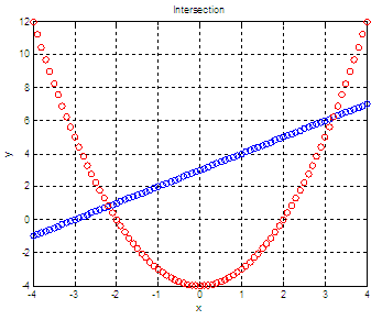
A figure that can better
display our discrete values is achieved
by using
plot(x,y1,'bo', x,y2,'ro')
The resulting figure
(showing discrete increments) is:

What I mean is that if we divide each element of one
function by the corresponding element of the other function, we’re not
going to
get exactly 1 at the intersections. We may try to find a good
approximation if
we look for quotients going from 0.95 to 1.05.
We may code something
like this:
d
= y1
./ (y2 + eps);
ix =
find(d > .95 & d < 1.05);
x_sol =
x(ix)
y1_sol =
y1(ix)
y2_sol =
y2(ix)
We addd an ‘eps’ to the y2 (in the first line) to avoid a
division by zero. ‘eps’ is a predefinded constant and is the smallest
number
that we can have in Matlab.
The results are:
x_sol =
-2.2000
3.2000
y1_sol
=
0.8000 6.2000
y2_sol
=
0.8400 6.2400
Note that y1 and y2 are not exactly
the same, but close.
Third approach. Subtract element-by-element.
Another approach to find
intersections is to
subtract the corresponding elements
of the functions. Naturally, we’re not going to find exact zeros at the
intersections. We can try, for example, differences of +/- 0.1. Let’s
try this code:
s = y1 -
y2;
ix =
find(s > -.1 & s < .1);
x_sol =
x(ix)
y1_sol =
y1(ix)
y2_sol =
y2(ix)
The results are:
x_sol
=
-2.2000 3.2000
y1_sol
=
0.8000 6.2000
y2_sol
=
0.8400 6.2400
Now, if we need more
accuracy, we could start by defining a
more continuous x-vector.
Instead of 0.1 increments, we might use 0.001
increments, and we could improve our 'specs' or tighten the closeness
to 1 for the division of
functions, and the closeness to 0 for their subtraction.
Now, find intersections
with Polar coordinates
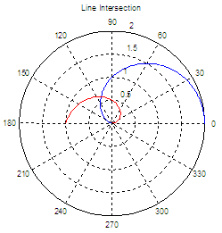
Another example. Let’s say that we need to find the
intersection of lines on this polar
graphic. We know beforehand the functions
that produce those lines.

Explore
the following code. We use a subtraction between lines, point-by-point.
When we find a difference very close to zero, we assume it's an
intersection because those two points are the same. This is not an
accurate concept, but a practical idea.
clear,
clc
%
define your angle
t = 0 :
0.001 : pi;
%
define your functions
r1 = 1 +
cos(t);
r2 =
t/pi;
%
plot
polar(t,
r1,'b')
hold on
polar(t,
r2, 'r')
title('Line
Intersection')
%
Intersection occurs when r1 - r2 = 0
%
Since your function is not continuous,
%
your result is an approximation
r = r1 -
r2;
%
find appropriate or best indices
ix =
find(r > -.001 & r < .001);
%
show results
disp('Magnitude
aprox: ')
rho1 =
r1(ix)
rho2 =
r2(ix)
disp('Intersection
aprox. at: ' )
radians
= t(ix)
degrees
= t(ix)*180/pi
The results are:
Magnitude aprox:
rho1 =
0.6233
0.6224
rho2 =
0.6229
0.6233
Intersection aprox. at:
radians =
1.9570
1.9580
degrees =
112.1278
112.1851
There’s only one
solution, we know. But since we’re finding
differences between -0.001 and 0.001, more ‘results’ are possible. From
the numerical point of view, those results are the same.
From
'Find Intersections'
to Matlab home
From
'Find Intersections' 'Matlab Programming'


|


