Impulse function - Dirac Delta

It's defined as follows:

The function depends on real input parameters. The function output is infinite when the input is exactly 0. The output is zero for any other input value. 

The Dirac delta is not strictly a function, because any real function that is equal to zero everywhere but at a single point must have a total integral equal to zero, but for many purposes this definition can be manipulated as a function.
 

Let’s create some discrete plots using Matlab function 'stem'.

 
For our purposes, we are going to define the function as 1 when the argument of the Dirac function is 0, and the output will be 0 for any other value of the input argument. 

We can define the function having a scalar as an input. For example:
 

function y = dd1(n)
% Our default value is 0
y = 0; 

% The function is 1 only if the input is 0
if n == 0
    y = 1;
end

Let’s find the appropriate output for this vector: 

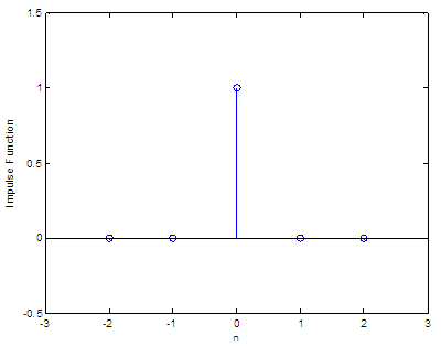
n = -2 : 2

We use our function above (‘dd1’) like this: 

for i = 1 : length(n)
    f(i) = dd1(n(i));
end
stem(n, f)
axis([-3 3 -.5 1.5])
xlabel('n')
ylabel('Impulse Function') 

The result, as expected, is:

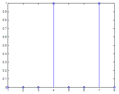
Now, let’s assume another vector:
 

n = [1 2 3 0 2 5 0 1]

 
We can use our function ‘dd1’ to find the delta function output: 

for i = 1 : length(n)
    f(i) = dd1(n(i));
end
stem(f)
 

The result is:

Now, let’s say that we have a vector (not a scalar) as an input. We want to calculate the unit function for all of the values included in the input vector. We can create another function ('dd') to considerate this approach:
 

function y = dd(x)
% x is a vector
% We create an output vector of only 0 (our default value)
y = zeros(1, length(x)); 

% We find indexes of input values equal to 0,
% and make them 1
y(find(x==0)) = 1;

 
We don’t need a loop now, so our process has been simplified a lot.
 

n = [1 2 3 0 2 5 0 1]
f = dd(n)

 
The result is: 

f = 0     0     0     1     0     0     1     0

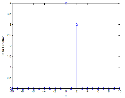
If we want to calculate y = 4δ(n) + 3δ(n-2), in a range of integers that go from -10 to 10, we can do simply this:
 

n = -10 : 10
y = 4*dd(n) + 3*dd(n-2)
stem(n, y)
xlabel('n')
ylabel('Delta Function')
 

and the result is:

We can see that every term in the function only counts as one stem, and that happens when the argument is zero. The first term, 4δ(n), has a height of 4 (coefficient) at n = 0; the second term, 3δ(n-2), has a magnitude of 3 (coefficient) at n = 2.