

WinSpice and Matlab: automation of electronic simulationsIn this article, a Matlab routine to drive the WinSpice circuit simulator is presented. This method can be easily adapted to simulate and drive any circuit entered in this SPICE version. The performance of the Matlab driver is illustrated by simulating a typical amplifier circuit using some resistors, capacitors and a transistor. In this example we're using Matlab ver. 7.0.1 and WinSpice3 ver. 1.04.07. For more information about Matlab, visit www.mathworks.com. For more information about WinSpice, visit www.winspice.com. SPICE stands for Simulation Program with Integrated Circuit Emphasis Interchanging information between Matlab and WinSpice allows the implementation of mathematical or optimization algorithms and graphical possibilities not included in the circuit simulator environment itself. The approach developed here is very flexible and utilizes the inherent capability of this SPICE simulator to execute text files and print data to external .csv (comma separated values) files. First, the circuit in Spice is defined (.cir file). This circuit is simulated and tested within the WinSpice environment before any attempt is made to interact with Matlab. Second, we prepare the output of the simulator by writing necessary data to an external file, that is, we include 'write' commands in the .cir file, so that the results are saved as external (.csv) text files available to Matlab. Third, we now generate a new version of the .cir file using Matlab capabilities for manipulating cell-arrays (string matrices), we then insert a Matlab statement to run the Spice simulator from the command line with the .cir filename as a parameter. After the simulation, we can read the results in the .csv files, process them and act accordingly. First Step: We create, test and simulate this circuit in WinSpice: 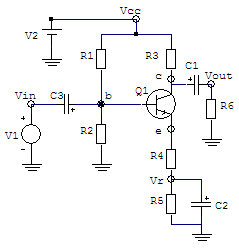 We use these values: R1 = 10k ohms, R2 = 5k ohms, R3 = 1k ohm, R4 = 50 ohms, R5 = 1k ohm, R6 = 3k ohms C1 = C2 = C3 = 10 uF Q1 = transistor 2N2222 V1(ac) = 0.1V amplitude @ 1k Hz V2(dc) = 30 V The .cir file (text file) needed is: --- Simple amplifier with Transistor ---- V1 Vin 0 dc 0 ac 1 sin(0 0.1 1e3) V2 Vcc 0 dc 30 R1 Vcc b 10e3 R2 b 0 5e3 R3 Vcc c 1ek R4 e Vr 50 R5 Vr 0 1e3 R6 Vout 0 3e3 C1 c Vout 10e-6 C2 Vr 0 10e-6 C3 b Vin 10e-6 Q1 c b e Q2N2222 .MODEL Q2N2222 NPN +(IS=3.108E-15 XTI=3 EG=1.11 VAF=131.5 BF=217.5 + NE=1.541 ISE=190.7E-15 IKF=1.296 XTB=1.5 BR=6.18 + NC=2 ISC=0 IKR=0 RC=1 CJC=14.57E-12 VJC=.75 + MJC=.3333 FC=.5 CJE=26.08E-12 VJE=.75 MJE=.3333 + TR=51.35E-9 TF=451E-12 ITF=.1 VTF=10 XTF=2) .control AC DEC 10 10 10MEGHZ plot vdb(Vout) TRAN 10E-6 5E-3 plot v(Vout) .endc .end The AC and Transient analysis deliver these results: 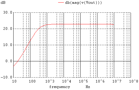 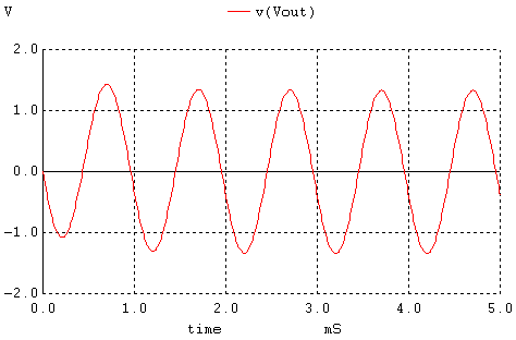 Second Step: We include appropriate 'write' commands in the .cir file, so that the results are saved as .csv files available to Matlab. The control block changes into: .control AC DEC 10 10 10MEGHZ write f_ac_out.csv vdb(Vout) TRAN 10E-6 5E-3 write f_tran_out.csv v(Vout) quit .endc .end Third Step: We now create a function (to be run by Matlab) that can reproduce the above .cir file (simulation of the amplifier), modify relevant parameters with the command 'num2str' (which changes numbers into strings), and launch the circuit simulator. This is the full code that accomplishes it: function [Rac
Rtran] = spice_amp(x) b{1} = ['-------------Simple
amplifier with Transistor----------- ']; %
Save file .cir line-by-line %
Run WinSpice %
Read data saved in .csv files function [Rac
Rtran] = getWSpicedata(WSpiceBaseFile) ac =
fopen([WSpiceBaseFile '_ac_out.csv']); tran =
fopen([WSpiceBaseFile '_tran_out.csv']); fclose('all'); Now, we're ready to perform some simulations driving WinSpice from Matlab. clear;
clc; close all %
We try some initial resistors %
Matlab launches the simulator including our parameters figure %
We try another gain modifying one of the resistors figure For R3 = 1k and R4 = 50, the obtained results are: 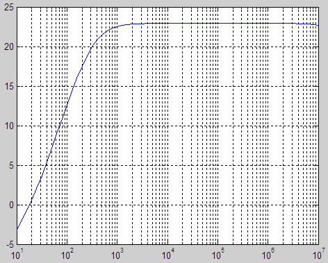 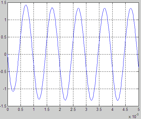 For R3 = 500 and R4 = 50, the obtained results are: 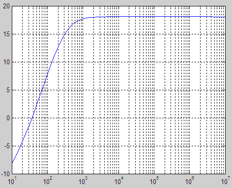 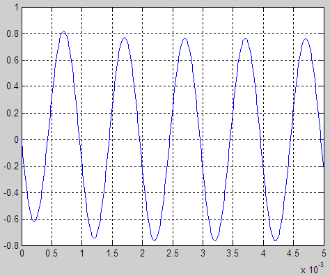 We can now use WinSpice as if it was another built-in Matlab function! This means that we can work through circuit optimization using Matlab... We can try some numbers in our design, we can see the results and use Matlab to modify relevant values in the circuit, in iterations. Very powerful, isn't it? Reference: http://desi.iteso.mx/erayas/cad.htm, 2014. See a variation of this technique From 'WSpice' to home From 'WinSpice' to Matlab Programming
|
